Utilizing the Accounting Number Format in Excel. Excel serves as a fundamental tool in business and accounting, often handling data sets primarily composed of numbers. To enhance clarity and tailor the data specifically for accounting purposes, users might opt to convert these numbers from their standard format to an accounting number format.
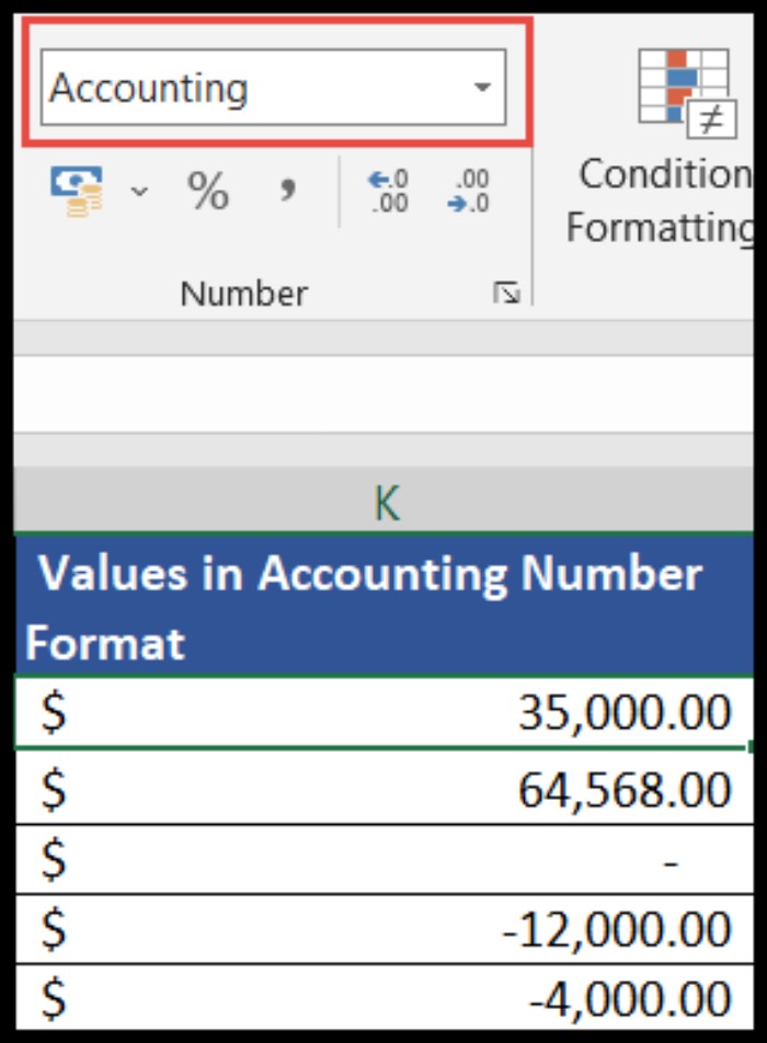
The accounting number format undergoes a transformation from the general number format by incorporating essential elements: placing the currency symbol at the far left of the cell, integrating thousand number separators, and ensuring each number concludes with precisely two decimal places (0.00).
Moreover, the accounting number format in Excel cleverly displays zero (0) values as a dash “-”.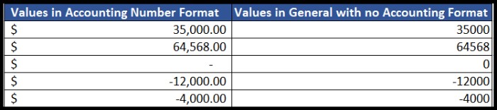
Utilizing the Accounting Number Format in Excel
Here are streamlined steps for effortlessly applying the accounting number format in Excel:
Applying Accounting Number Format Using the Accounting Number Format Button
- Select Desired Cells Highlight the cells or range housing the numbers you wish to format.
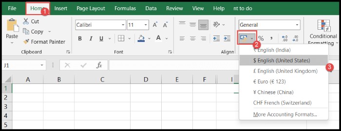
- Access the “Home” Tab Navigate to the “Home” tab and locate the “Accounting Number Format” button.
- Select Currency Format Click the button and choose the preferred accounting format featuring the desired currency symbol from the provided drop-down list.
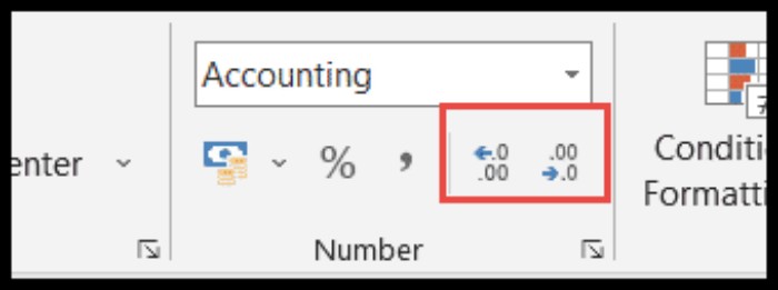
- Adjust Decimal Values For adjusting decimal values, utilize the “Increase” or “Decrease” icons under the “Number” group on the ribbon.
Applying Accounting Number Format Using the Drop-Down in the Number Group
- Select Desired Cells Highlight the cells or range containing the numbers for formatting.
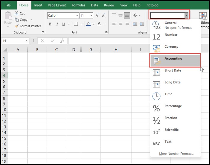
- Access the “Home” Tab Proceed to the “Home” tab and click the drop-down arrow under the “Number” group.
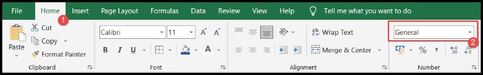
- Choose Accounting Format From the drop-down list, opt for the “Accounting” option.
Applying Accounting Number Format Using the Format Cells Option
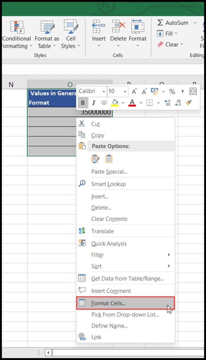
- Select Desired Cells Highlight the cells or range containing the numbers requiring formatting, then right-click the selection.
- Access “Format Cells” Choose the “Format Cells” option from the ensuing drop-down menu to open the “Format Cells” dialog box.

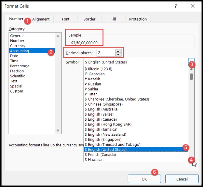
- Navigate to “Number” Tab Within the “Format Cells” dialog box, select the “Number” tab and then choose “Accounting” from the “Category” list.
- Customize Currency Symbol Click the drop-down arrow next to “Symbol” to explore and select your desired currency symbol. Adjust decimal places if necessary.
- Finalize Changes Confirm your selections by clicking “OK.”

By following these straightforward methods, users can seamlessly convert their number sets into the accounting number format, incorporating specific currency symbols and decimal preferences for enhanced clarity in Excel.