Modifying Pivot Table Data Source in Excel. Efficiently managing changing data sources for your Pivot Table is crucial. Here’s a straightforward guide on adjusting or locating the data source dynamically:
Modifying Pivot Table Data Source in Excel
- Begin by clicking anywhere on the pivot table to activate the “Analyze” tab.
- Navigate to the “Analyze” tab.
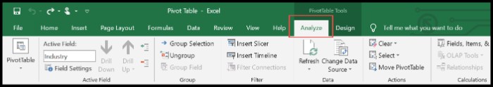
- Click on the “Change Data Source” option under the “Data” section.

- A “Change PivotTable Data Source” dialog box will appear.
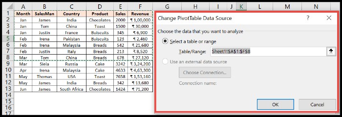
- In the dialog box, identify the current data range, ensuring all relevant data is included. Update the range by selecting the complete data (e.g., Sheet1!$A$1:$F$13) or using the table name range.
- Click “OK” to apply the updated data source.
Additionally, you can use the shortcut key Alt ⇢ J ⇢ T ⇢ I ⇢ D to directly open the “Change PivotTable Data Source” dialog box.
Modifying Pivot Table Data Source in Excel. For a more streamlined process, consider converting your source data into an Excel Table using the shortcut Ctrl + T. This eliminates the need for frequent data source updates; refreshing the Pivot Table will automatically incorporate any changes.