Managing Pivot Table Data Sources in Excel. In this guide, we’ll explore the essential process of altering or locating the data source for a particular Pivot Table in Excel. This capability proves incredibly valuable, especially when your dataset undergoes frequent changes.
Managing Pivot Table Data Sources in Excel: A Step-by-Step Guide
Follow these comprehensive steps to efficiently manage your data sources:
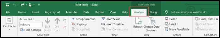
- Activate the Analyze Tab: Start by clicking anywhere within the pivot table to activate the ‘Analyze’ tab.
- Access the Change Data Source Option: Navigate to the ‘Analyze’ tab and locate the ‘Change Data Source’ option under the ‘Data’ section.
- Adjust the Data Source: Upon clicking, a dialogue box labeled ‘Change PivotTable Data Source’ will appear. Here, you’ll observe the current data range assigned to the PivotTable, such as ‘Sheet1!$A$1:$F$8’, implying that rows A9 to A13 are excluded.

- Select the Updated Range: You can either manually select the complete updated data range, like ‘Sheet1!$A$1:$F$13’, or utilize the table name range to redefine your PivotTable’s data source.
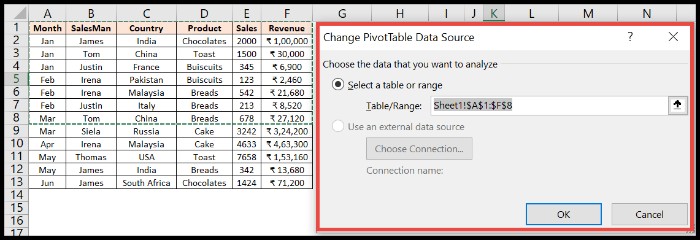
- Confirm Changes: To apply the modifications, click ‘OK’ within the dialogue box, thus updating the data source.
Additionally, for quicker access to the ‘Change PivotTable Data Source’ dialogue box, you can use the shortcut keys Alt ⇢ J ⇢ T ⇢ I ⇢ D.
An Efficient Tip: Always convert your source data into an Excel Table using the keyboard shortcut Ctrl + T. This conversion eliminates the need for recurrently updating your data source. A simple refresh of the Pivot Table will automatically incorporate any changes in the data range.
Managing Pivot Table Data Sources in Excel. By employing these techniques, you’ll streamline the management of your Pivot Table data sources, ensuring seamless updates and efficient data handling.