How to Highlight Rows in Excel Based on Specific Text. At times, pinpointing rows containing specific text becomes essential. In this guide, we’ll explore how to highlight a row if any cell within that row contains a particular text or value, leveraging conditional formatting.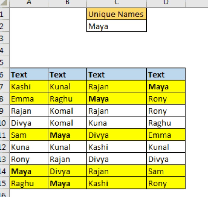
How to Highlight Rows in Excel Based on Specific Text
The formula we’ll use for conditional formatting involves the MATCH function:
=MATCH(lookup_value, lookup_array, 0)
Lookup value: This represents the text criterion we’ll be searching for within the specified range.Lookup array: Refers to the row that requires highlighting.- It’s crucial to select the first row when applying conditional formatting.
Example: Highlighting Rows Containing Specific Text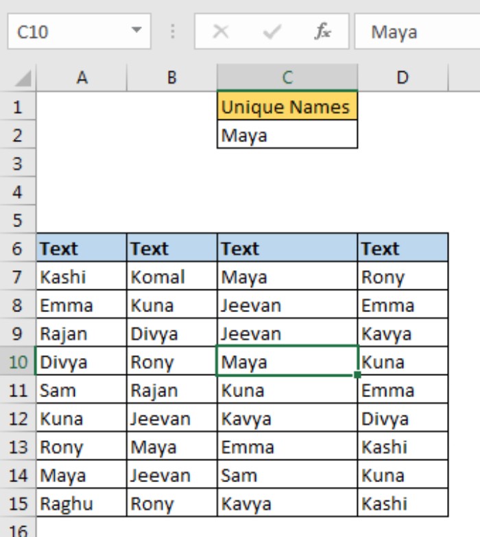
Let’s consider a dataset with various names in each row. Our goal is to highlight rows that contain the value in cell C2 (currently set as “Maya”).
- Select the first row of the table (A7:D7).
- Navigate to conditional formatting and create a new rule (shortcut: ALT > H > L > N).
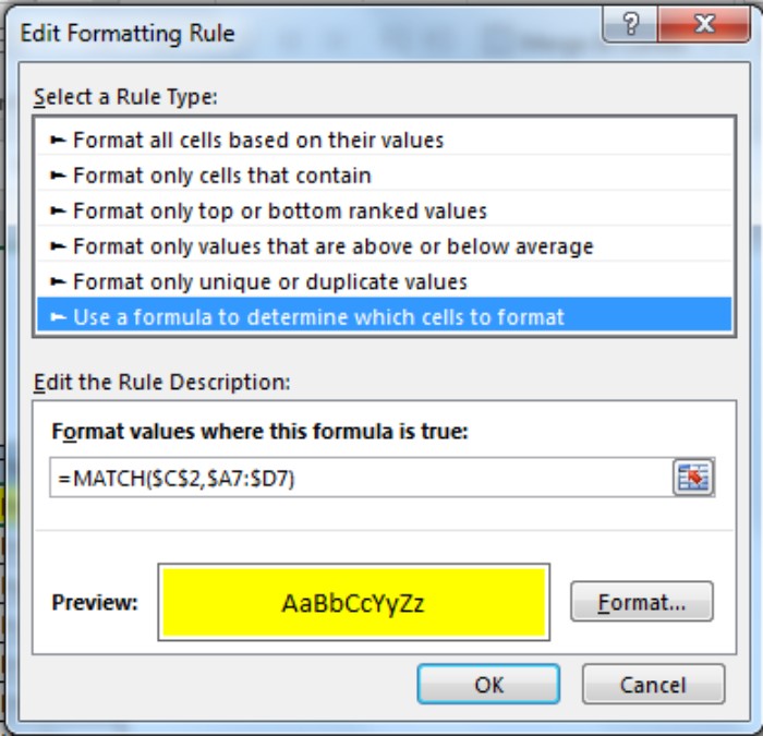
- Choose “use a formula to determine which cell to format.”
- Enter the formula:
=MATCH($C$2, $A7:$D7, 0)
- Select the formatting option (e.g., yellow fill) and confirm.
Now, the selected row will be highlighted.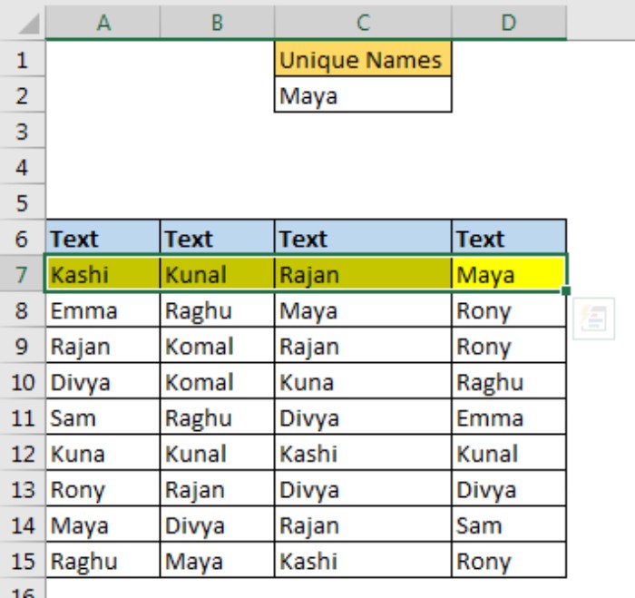 To extend this formatting to the entire table, copy the formatted range and apply it to the complete dataset.
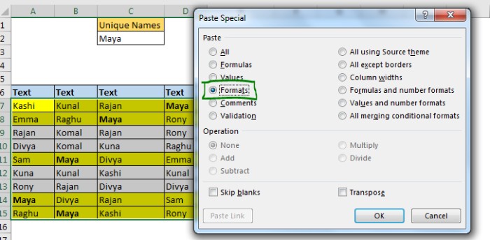
How It Functions: How to Highlight Rows in Excel Based on Specific Text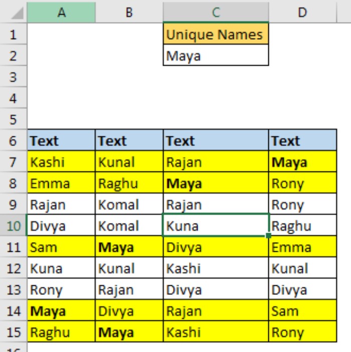
We utilize Excel’s MATCH function, which identifies the index of the sought-after value within the specified range. If the text is not found, it returns an #NA error.
In conditional formatting, positive values equate to TRUE, while errors translate to FALSE. Leveraging this behavior, our formula highlights rows based on the presence of specific text within any cell.
The formula =MATCH($C$2, $A7:$D7, 0) ensures the reference to the lookup value (C2) remains fixed, consistently searching for the value. The lookup range (A7:D7) maintains relative rows and absolute columns, enabling the adjustment of the lookup row while copying the conditional formatting.
Adjustments to the formula, such as making the columns relative, can result in highlighting rows based on the first-found value.
In instances where the goal is to check for text within strings, utilizing SEARCH($C$2, $A7&$B7&$C7&$D7) becomes pivotal. This function scans for the text in concatenated cells of A7:D7 and triggers conditional formatting based on the outcome.
Additionally, for case-sensitive matches, employing the FIND($C$2, $A7&$B7&$C7&$D7) function validates text and case within rows, ensuring accurate row highlighting.
How to Highlight Rows in Excel Based on Specific Text. This method provides a robust approach to highlight rows based on text matches in Excel. If any questions arise or you seek clarification on Excel/VBA-related topics, feel free to engage in the comments section below.