Cell Value in Excel. In a previous guide, we explored highlighting entire rows if any cell within them contained specific text. Now, let’s delve into highlighting rows based on a specific cell value. This method extends beyond text; we’ll utilize conditional formatting to highlight rows when certain criteria are met.
How to Highlight a Row Based on a Cell Value in Excel
The Generic Formula in Conditional Formatting
The formula we’ll employ in conditional formatting is:
=(cell with relative row = criteria)
Cell with relative row: This references a cell where the column remains fixed while the row is relative (e.g., $A1). You can explore referencing in Excel in detail [here](link to detailed reference guide).Criteria: This denotes the value or condition that triggers the row highlighting. It could be text, a value, or a logical test.
Example: Highlighting Rows Based on Fruit Rates
Suppose we have a fruit dataset and want to highlight entire rows where the fruit rate exceeds 100.
- Select the first row of the table (A2:C2).
- Navigate to conditional formatting and create a new rule (shortcut: ALT > H > L > N).
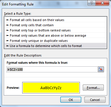
- Choose “use a formula to determine which cell to format.”
- Input this formula:
=$C2>100
Ensure the entire row is selected before applying conditional formatting.
- Select the formatting option (e.g., yellow fill) and confirm.
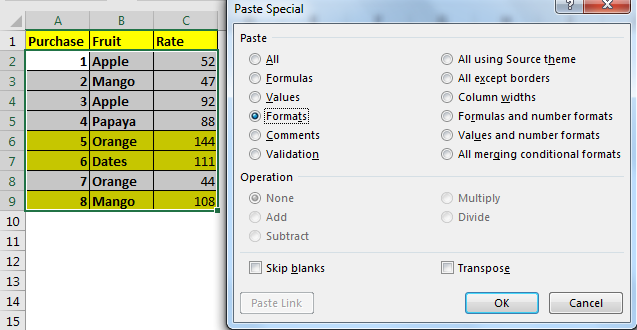
After applying this formatting to the selected range, copy it and paste the format across the entire table.
Now, each row with a fruit rate exceeding 100 will be highlighted. While I’ve set the criteria directly, you can also refer to a specific cell for this criterion.
How It Works
The process is straightforward: we check if the value in cell $C2 is greater than 100. When it satisfies this condition, Excel highlights the entire row.
Note that only column C is anchored using $. The rows remain relative as we intend to adjust the lookup row while copying the conditional formatting, keeping the columns fixed. Ultimately, this approach highlights rows containing values greater than 100.


