Creating Cascading Drop-Down Lists in Excel. In this guide, we’ll explore the process of creating cascading drop-down lists using conditional formatting. To establish these lists, we’ll rely on the Countif and Indirect functions.
Creating Cascading Drop-Down Lists in Excel
Let’s consider an example:
We’ve compiled a list of Fruits & Vegetables.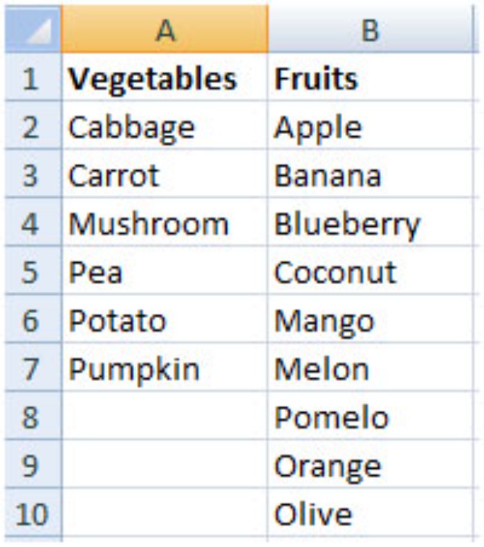
Our aim is to generate a cascading drop-down list that will highlight any incorrect selections (flagging values that don’t belong to Fruits or Vegetables).
We’ll follow these steps:
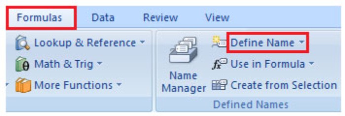
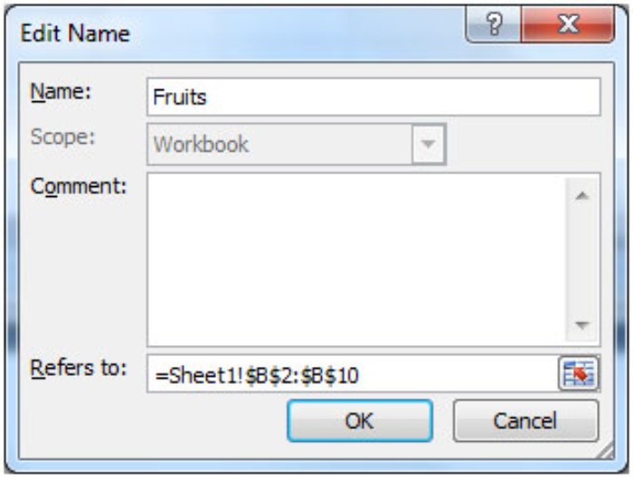
- Using Define Name, we’ll create named ranges for Vegetables & Fruits. img3

- The next stage involves setting up data validation lists for Fruits & Vegetables in the range A13:A18. Refer to the screenshot below.
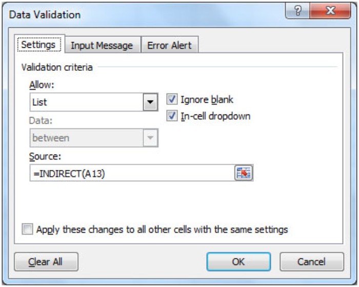
- In range B13:B18, we’ll establish data validation lists with a formula referencing cell A13 using the Indirect function.
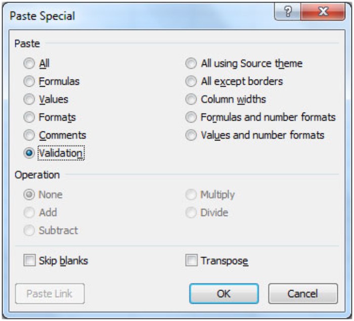
- Copy cell B13, then Paste Special and select Validation for the range B14:B18.
This will replicate the validation across the chosen cells.
Once the data validation process is complete, we can utilize a formula to flag incorrect selections.
- Select the range B13:B18.
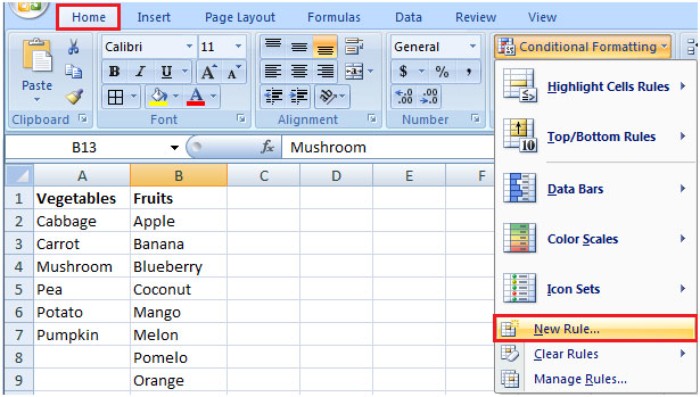
- Navigate to the Home tab and choose Conditional Formatting.
- Click on New Rule.
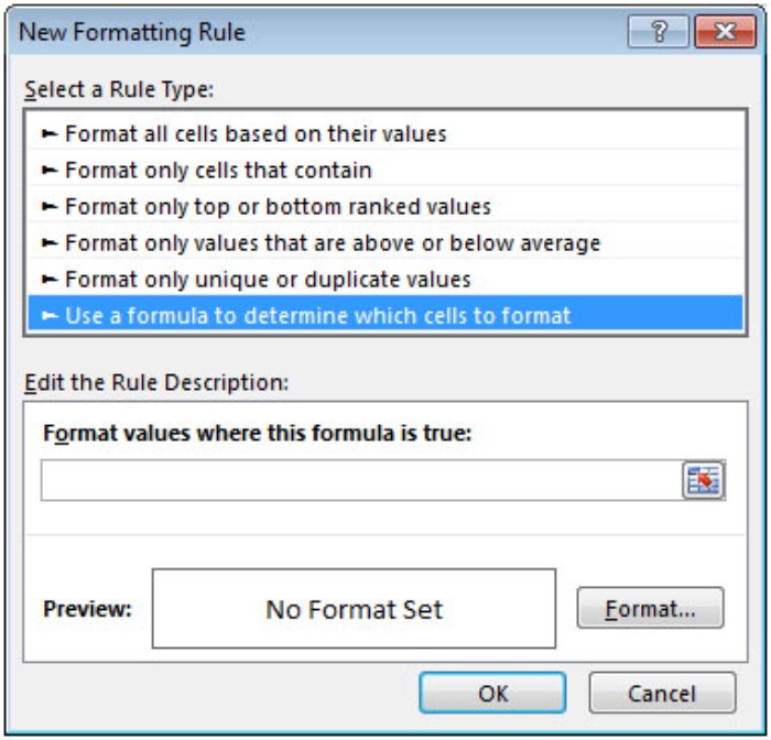
- In the New Formatting Rule dialog box, select “Use a formula to determine which cells to format.”

- Enter the formula =COUNTIF(INDIRECT(A13),B13)=0.
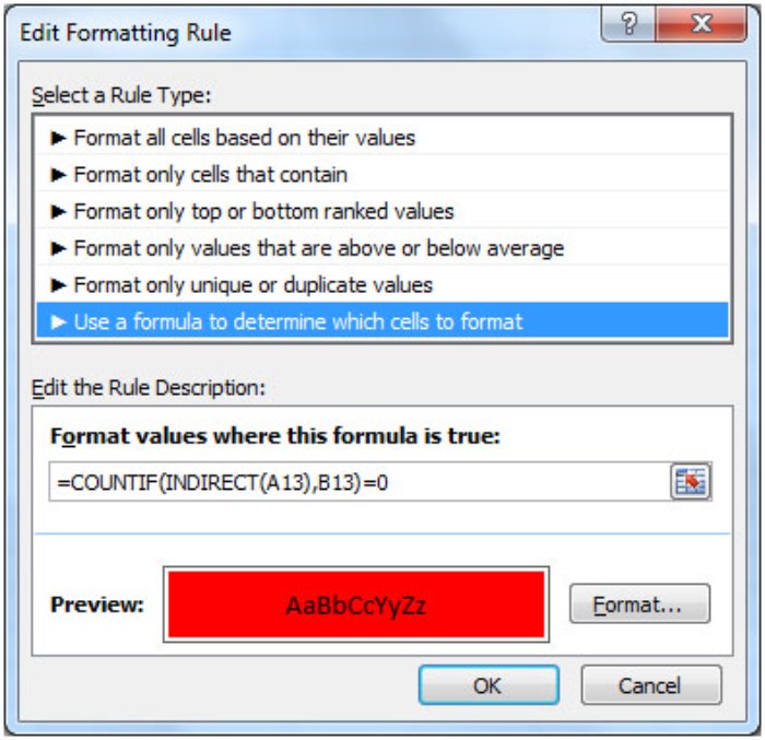
- Click on Format, configure the formatting, then click OK twice.

The following snapshot demonstrates everything in order. 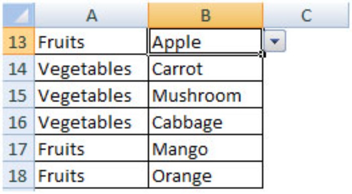
However, once we change Fruits to Vegetables in cell A13, you’ll notice the conditional formatting takes effect, highlighting the incorrect selection. 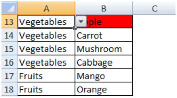
Likewise, altering the value in any dropdown below—let’s say cell A18—will also trigger a highlighting effect. 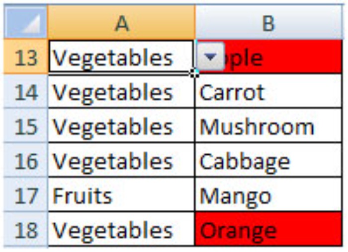
This method enables us to track and rectify incorrect selections made within the dropdown list.