Creating a Colorful Dropdown List in Excel

Creating a Colorful Dropdown List in Excel

Discover how to enhance your Excel spreadsheet by adding a dropdown list with colors. This article guides you through the process, utilizing Microsoft Excel‘s Conditional Formatting and Data Validation features.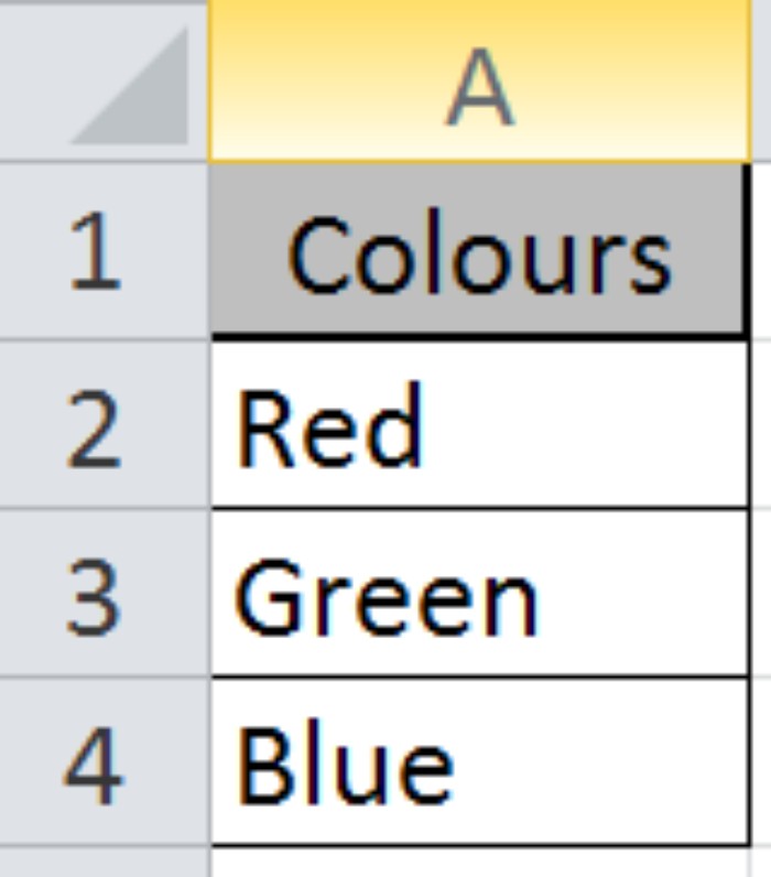

Steps to Create a Dropdown List:

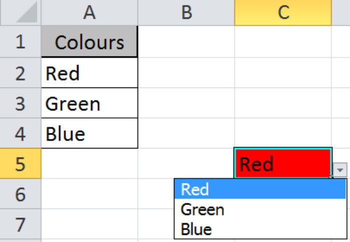
1. Begin with a list of colors, for example, Red, Green, and Blue.
2. Navigate to Data > Data Validation in Excel 2016.
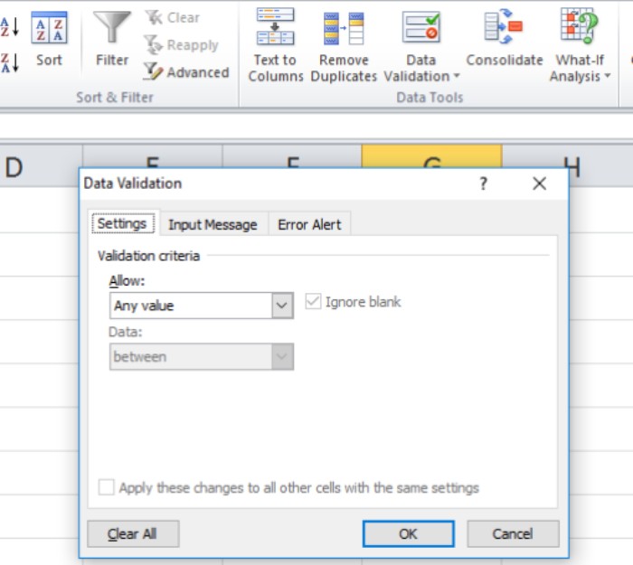
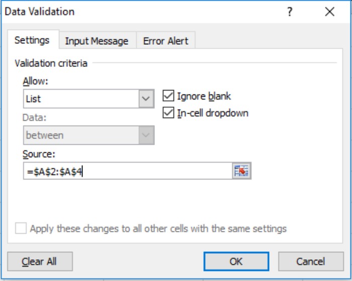
3. In the Data Validation dialog box, choose “List” in the Allow field, select the source list, and click OK.

A dropdown list is now created on the designated cell.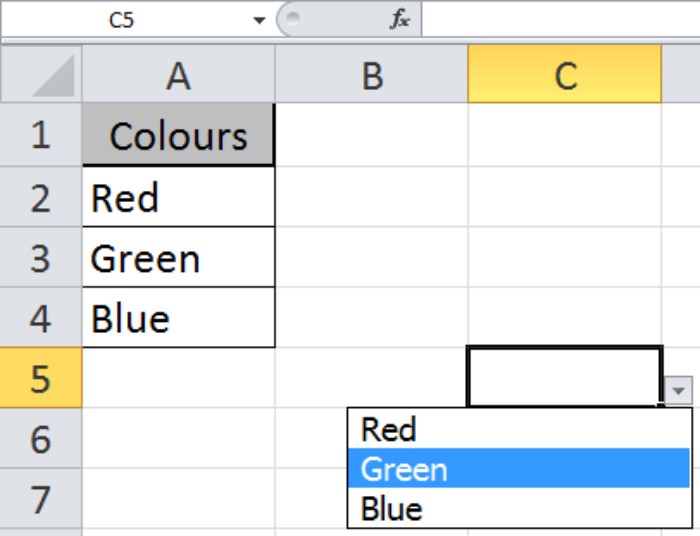

Applying Conditional Formatting:

1. Go to Home > Conditional Formatting and select “New Rule” from the list.
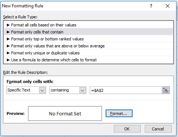
2. In the dialog box, choose “Specific Text” and select the cell corresponding to the color (e.g., Red).
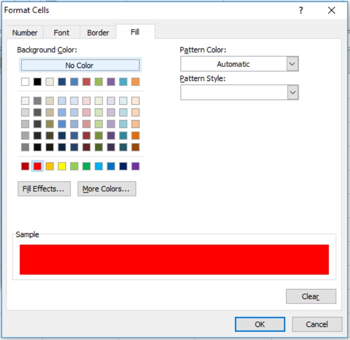
3. Select Format > Fill, pick the desired color (Red), and click OK.

Repeat this process for other options like Green and Blue.

Dropdown List in Excel. Your dropdown list, enhanced with conditional formatting, will provide a visually appealing representation of your data. These tools are valuable in Excel 2016 for presenting and organizing information. Note that you can apply a similar method to create a dropdown list in Google Sheets.