Utilizing SUMIF Function in Excel for Non-Blank Cells. In this guide, we will delve into the process of obtaining a return from non-blank cells using the SUMIF function in Excel.
When you find yourself in need of applying the SUMIF function with specific conditions, the SUMIF function becomes invaluable. It calculates the sum of a range based on a given condition and returns the resulting values.
Utilizing SUMIF Function in Excel for Non-Blank Cells
Syntax:
=SUMIF(range, criteria, [sum_range])
Let’s illustrate how to use the SUMIF function with an example:
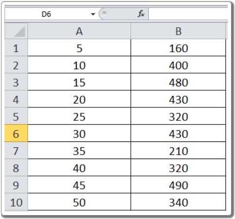
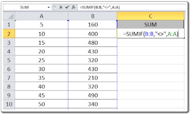
Suppose we want to use the SUMIF function to sum the numbers in column A only if the corresponding cell in column B is not empty. Here’s the formula:
=SUMIF(B:B, "<>", A:A)
Explanation: The formula assesses cells in column B that are not blank. If a cell is not blank, it captures the value from the corresponding cell in column A. The function ultimately returns the sum of these recorded values.
Example:
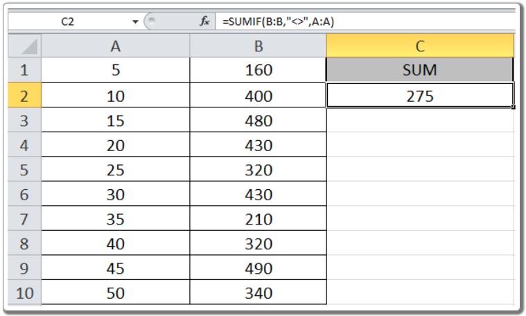
- Enter the formula where you want to obtain the sum.
=SUMIF(B:B, "<>", A:A)
- Press Enter to calculate and obtain the desired result.
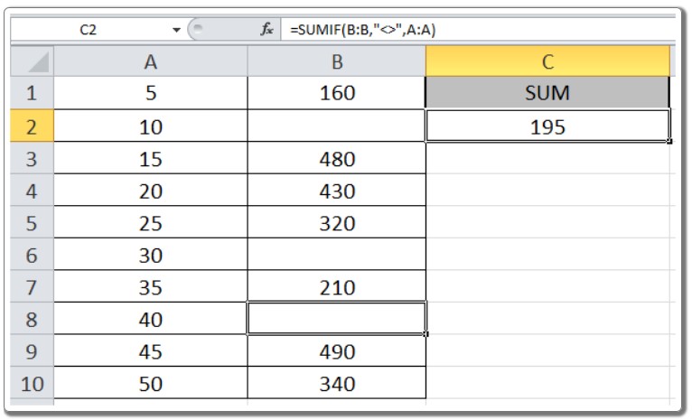
- Adjust the content in Column B by removing some numbers.
- Notice that as numbers are removed, the sum dynamically changes. The formula considers only non-blank cells in Column B, providing the sum of corresponding values in Column A.
By learning how to use the SUMIF function in Excel, you gain the ability to retrieve returns based on non-blank cells. This technique is applicable across Excel 2016, 2013, and 2010. Explore more articles on mathematical formulations with conditions here. If you encounter any issues or have unresolved queries, feel free to comment below.