Mastering Histograms in Excel. In this comprehensive guide, we’ll explore the process of creating XY graphs in Excel, commonly known as scatter charts or XY charts. These charts offer a direct visualization of trends and correlations between two variables, allowing for a clear understanding of their relationship. This tutorial covers everything from plotting X vs. Y data points to adding axis labels, data labels, and various other valuable tips.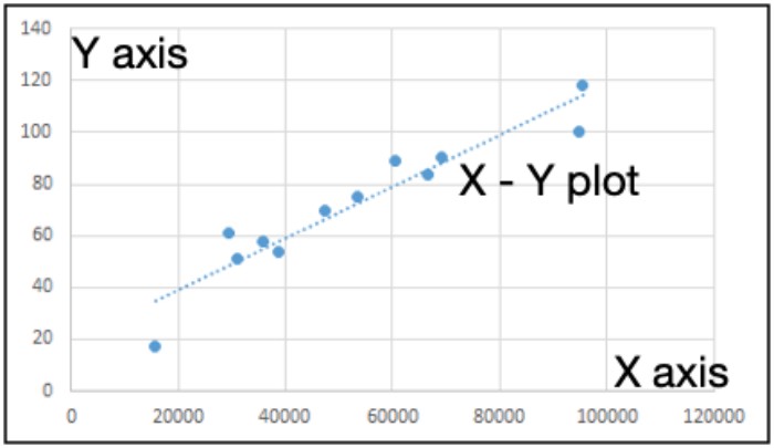
Mastering Histograms in Excel: A Step-by-Step Guide
Understanding Scatter Plots in Excel
Scatter charts in Excel are invaluable tools for revealing relationships between variables. By utilizing these charts, you can easily discern how one variable affects others. Visualizing correlations between different sets of data becomes effortless, enabling you to add trendlines for future value estimations.
Mastering Histograms in Excel: Example Scenario
Let’s illustrate this process with an example. Imagine you have data representing advertising costs (X) and corresponding sales figures (Y). To understand the impact of advertising costs on sales, you can create a scatter plot in Excel.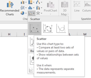
Creating Scatter Plots in Excel: Step by Step
- Select the Data: Choose the two variables you want to compare (e.g., Ad Cost and Sales). Select the corresponding data range (e.g., B1:C13).

- Insert Scatter Chart: Navigate to Insert > Charts > Scatter > Select Scatter.Your chart is now generated.
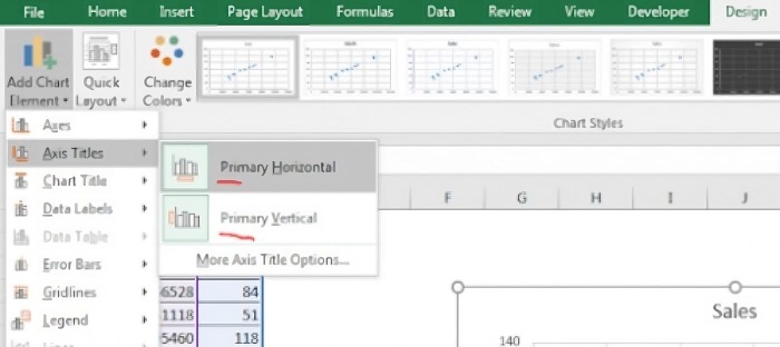
- Adding Axis Labels: To enhance clarity, add axis labels.
- Select the scatter plot.
- Go to the Design Tab.
- Click on Add Chart Element.
- Choose Primary Horizontal and Primary Vertical one by one.
- Rename them as “Ad Cost” and “Sales” respectively.
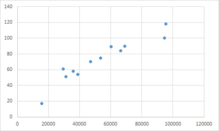
Your chart is now more readable and informative.
- Adding Trendlines: Trendlines provide valuable insights into your data.
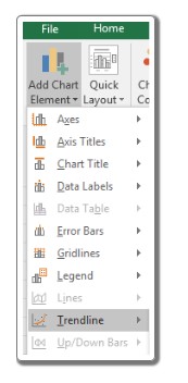
- Select the scatter plot.
- Go to Design Tab.
- Click on Add Chart Element.
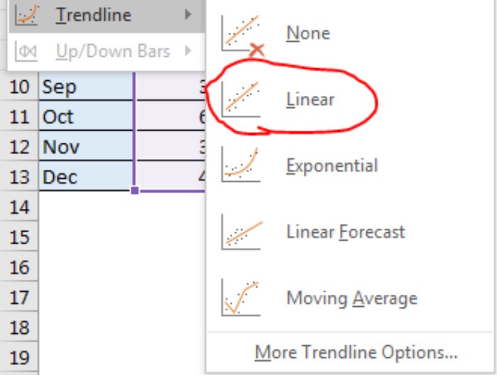
- Select Trendline.
- Choose Linear.
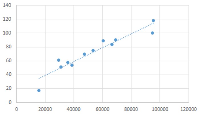
Your chart now displays the trendline, offering a clear visualization of the data’s trajectory.
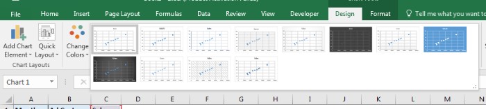
- Customizing Scatter Chart: Excel provides various customization options for scatter plots.
- Explore different chart styles under Chart Styles.
- You can manually set intercepts by checking the “Set Intercept” option above the Display Equation on the chart.
Mastering Histograms in Excel: Additional Tips and Notes
- Equations and Interpretations: You can add equations, intercepts, and slopes to the plot, enhancing its comprehensibility.
- Exploring Further: Delve deeper into scatter plots and explore other Excel chart types to broaden your data visualization skills.
Mastering Histograms in Excel. We hope this guide on How To Plot X Vs Y Data Points In Excel has been illuminating. For more articles on value calculations and related Excel formulas, stay tuned. Happy charting!