Highlighting the First Cell Based on Row Criteria
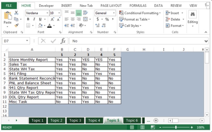
Highlighting the First Cell Based on Row Criteria. Here’s a more streamlined set of instructions for highlighting cells in Excel based on task completion:
- Select Column A.
- Click on “Conditional Formatting” and choose “Manage Rules”.
- In the dialog box, select “New Rule” and opt for “Use a formula to determine which cells to format.”
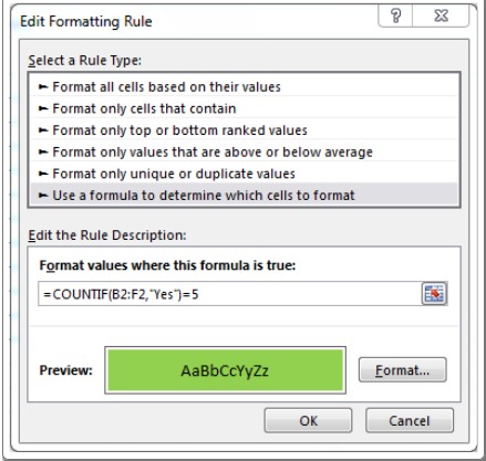
For cells turning Green (indicating completed tasks):
- Enter the formula:
=COUNTIF(B2:F2,"Yes")=5 - Click “Format” and choose the Green color.

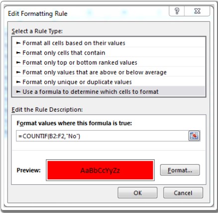
For cells turning Red (indicating incomplete tasks):
- Enter the formula:
=COUNTIF(B2:F2,"No") - Click “Format” and select the Red color.

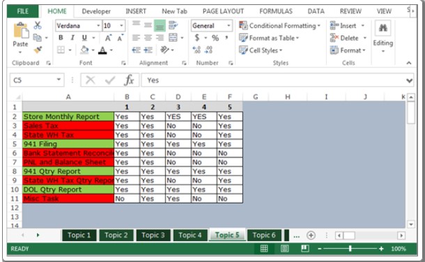
Click “OK”, then “Apply”, and finally, “OK” again to implement the conditional formatting. This setup will highlight cells in Column A based on the completion status of tasks listed across columns B to F. Highlighting the First Cell Based on Row Criteria


