Excel: Translate Column Letters to Numbers. In a prior tutorial, we explored converting column numbers to letters. But what about going the other way, transforming column letters into numbers? In this guide, we’ll uncover the process for converting Excel columns to numbers.
Let’s dive into a function called COLUMN, which retrieves the column number from a specified reference. We’ll combine the COLUMN function with INDIRECT to extract the column number from a given column letter.
Excel: Translate Column Letters to Numbers
Generic Formula to Convert Letters to Numbers in Excel
=COLUMN(INDIRECT(col_letter & “1”)) (col_letter): This references the column letter from which you want to extract the column number.
Example: Building an Excel Column Letter to Number Converter
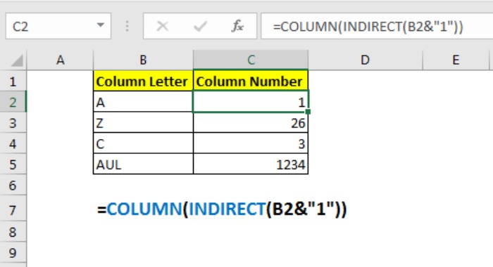
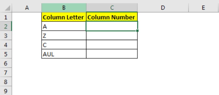
Consider a range of column letters in B2:B5. Our aim is to fetch the corresponding column numbers (1, 2, 3, and so on) from these given letters (A, B, C, and so forth).
Apply the aforementioned generic formula to obtain the column numbers for the given letters.
=COLUMN(INDIRECT(B2&”1″)) Drag the formula down across B2:B5. You’ll obtain the column numbers for the respective column letters.
How Does It Operate?
The concept is straightforward: it retrieves the reference of the first cell from the provided column number. Then, utilizing the COLUMN function, it extracts the column number from the given column letter.
For instance, INDIRECT(B2&”1″) translates to INDIRECT(“A1″), providing us the cell reference of A1. Consequently, COLUMN(A1) delivers the column number corresponding to the given column letter.
That’s the drill on converting a column letter into a column index number. It’s a straightforward process. If you have queries about this function or any other advanced Excel functions, feel free to share in the comments below.


