Excel Tips: Count/sum cells by color (background, font, conditional formatting)

October 23, 2023

16 Views 0

SaveSavedRemoved 0

In Excel, users often need to count or sum cells based on specific background colors. However, the standard Excel functions do not directly support this feature. To tackle this issue, we can utilize a User-Defined Function (UDF) in Excel VBA. Follow the steps below to create and implement this function:

Step 1:

Open the VBA module editor and copy the code

Press Alt + F11 to open the Microsoft Visual Basic for Application window.
In the newly opened window, click on “Insert” and then choose “Module” to create a new empty module.
Copy and paste the following VBA code into the empty module:

Function ColorFunction(rColor As Range, rRange As Range, Optional SUM As Boolean = False) As Variant
‘Updateby Extendoffice
Dim rCell As Range
Dim lCol As Long
Dim vResult As Double
lCol = rColor.Interior.ColorIndex
vResult = 0
If SUM Then
For Each rCell In rRange
If rCell.Interior.ColorIndex = lCol Then
vResult = vResult + rCell.Value
End If
Next rCell
Else
For Each rCell In rRange
If rCell.Interior.ColorIndex = lCol Then
vResult = vResult + 1
End If
Next rCell
End If
ColorFunction = vResult
End Function

Step 2:

Create the formulas to count and sum cells based on background color

After pasting the code, close the module window and apply the following formulas:

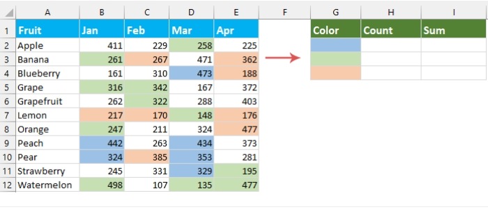
To count the number of cells with a specific background color: Copy or input the provided formula into the desired cell for the result. Then, drag the fill handle downwards to obtain results for other cells. See the screenshot:

=colorfunction(G2,$B$2:$E$12,FALSE)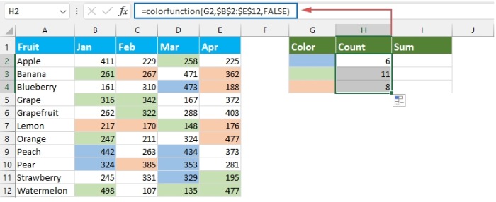

Count/sum cells by color

Note: In this formula, G2 represents the reference cell containing the specific background color you want to match; $B$2:$E$12 is the range where you want to count the cells with the corresponding color; FALSE is used to count the matching cells.

To sum the values of cells with a specific background color: Copy or input the provided formula into the desired cell for the result. Then, drag the fill handle downwards to obtain results for other cells. See the screenshot:

=colorfunction(G2,$B$2:$E$12,TRUE)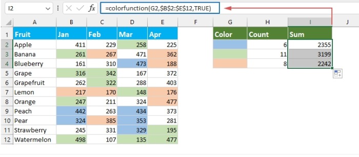

In this formula, G2 represents the reference cell containing the specific background color you want to match; $B$2:$E$12 is the range where you want to sum the values of cells with the corresponding color; TRUE is used to sum the values of matching cells.