Efficient Multiple Dropdown Lists in Excel. In this comprehensive guide, we’ll delve into the creation of multiple dropdown lists in Excel without repetitive entries, leveraging the power of Named Ranges.
Efficient Multiple Dropdown Lists in Excel
What are dropdown lists in Excel?
Dropdown lists serve as a tool to limit data manipulation within an Excel sheet. They restrict users to select values solely from predefined options, aiding in data validation. 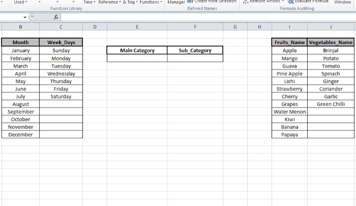 Multiple dropdown lists intertwine one selection with subsequent choices. For instance, choosing a week from the initial list narrows down options to specific weekdays, while selecting ‘fruits’ refines the subsequent list to fruit names, excluding weekdays.
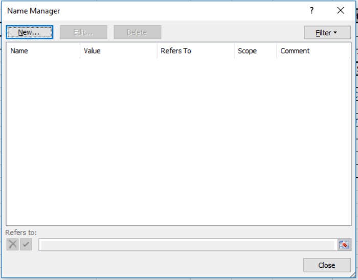
Illustrative Example:
Before delving into complexities, let’s grasp the process through an example: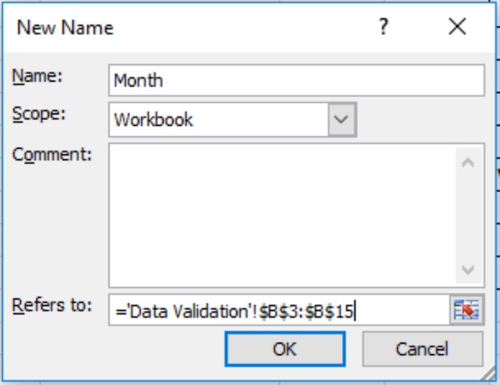
Consider the following lists:
To initiate, create a dropdown list for the ‘Main Category,’ leading to the ‘Sub_Category.’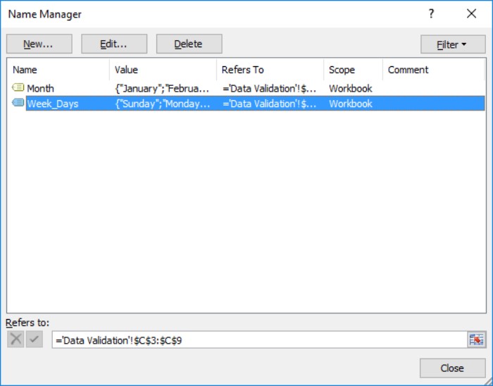
Begin by accessing Formula > Name Manager or using the Ctrl + F3 shortcut to open Name Manager. Here, define arrays with respective names to be easily referenced.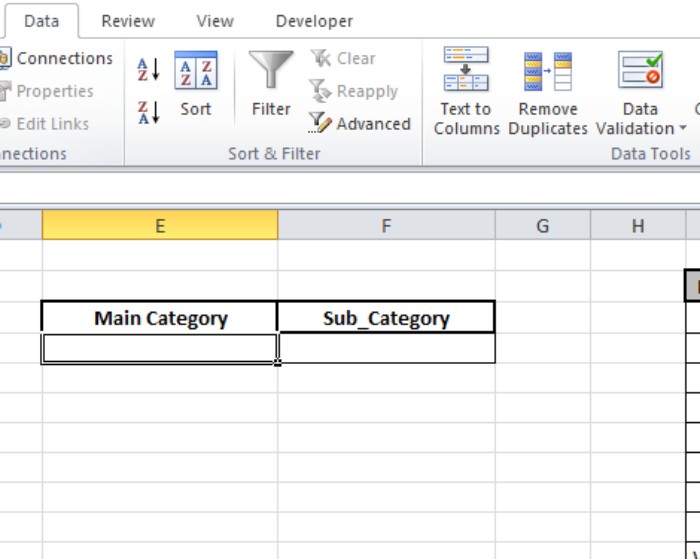
Create new lists like ‘Month’ and ‘Week_Days’ within Name Manager, ensuring accurate data references.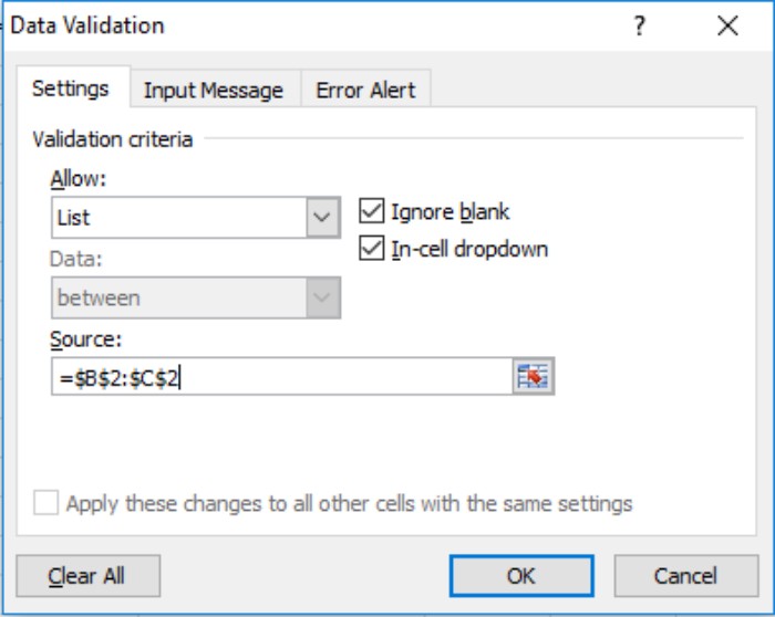
Close the manager and select the desired cell for the dropdown list.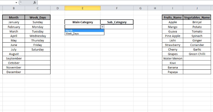
Navigate to Data Validation under the Data bar, choosing ‘list’ in the ‘Allow’ field and selecting cells containing ‘Month’ and ‘Week_Days’ categories (e.g., B2 and C2 cells).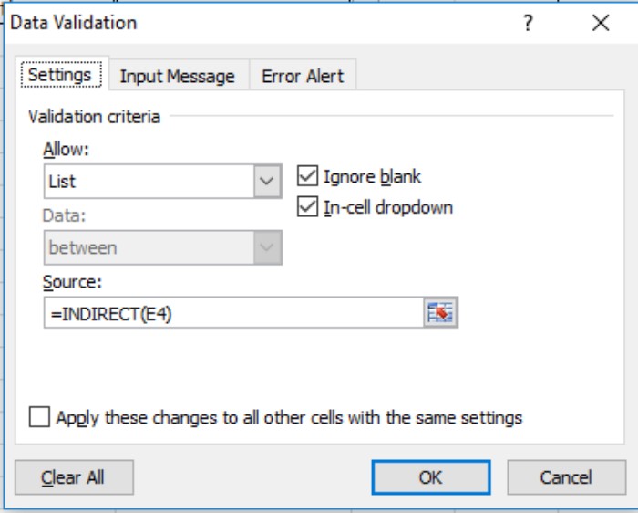
This action establishes a dropdown list for user selection.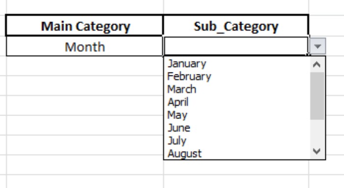
Next, proceed to the ‘Sub_Category’ cell and input the following formula in Data Validation, then click OK: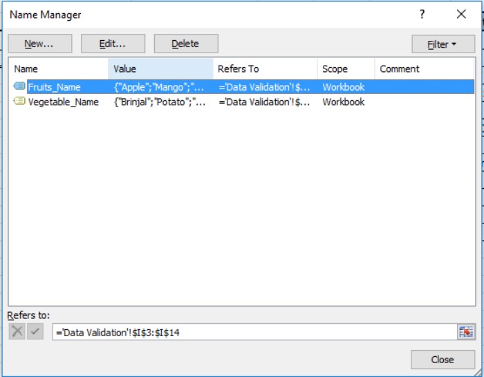
=INDIRECT(E4)
Resulting in:
If you wish to switch from ‘Month’ and ‘Week_Days’ to ‘Fruits_Name’ and ‘Vegetables_Name,’ simply modify the Name Manager lists.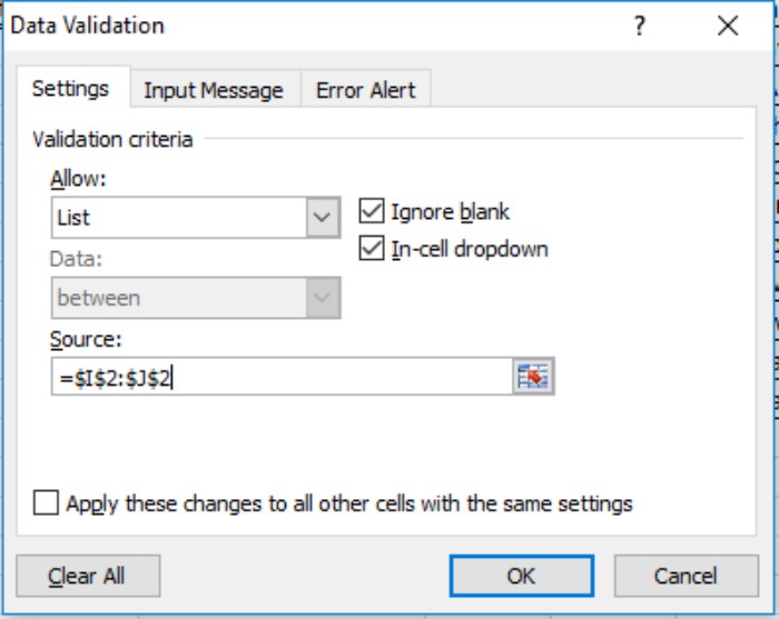
Open Name Manager (Ctrl + F3), delete existing lists, and introduce the new lists—’Fruits_Name’ and ‘Vegetables_Name.’
In Data Validation under ‘Sub_Category,’ substitute ‘Fruits_Name’ and ‘Vegetables_Name’ for ‘Month’ and ‘Week_Days,’ then click OK.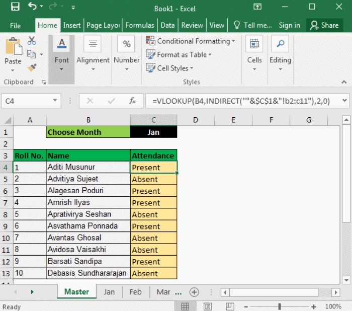
Witness the updated dropdown list options.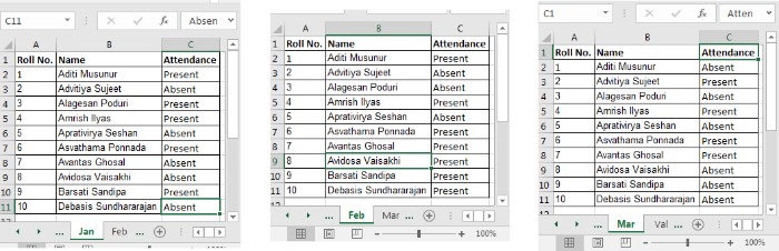
Additionally, let’s explore an alternative scenario:
Imagine being a teacher maintaining students’ attendance records across various monthly sheets within a workbook. To check individual attendance, a VLOOKUP is essential, even across different sheets.
Create a dropdown in Cell C1, containing a list of months.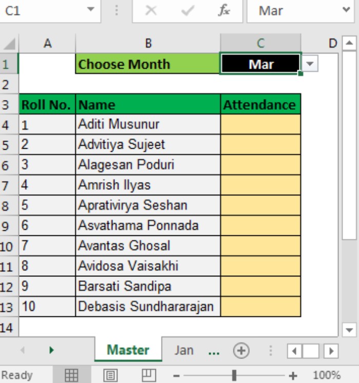
Utilize the generic formula for VLOOKUP from Multiple Sheets:
=VLOOKUP(lookupValue,INDIRECT(“”&cell with the month’s name&”!range”),col_index_no,0)
For instance, attendance data for “Jan,” “Feb,” and “Mar” resides within the range A2:C11 across respective sheets.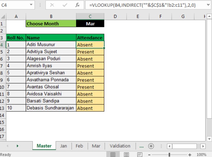
On the master sheet, input the VLOOKUP formula in Cell C4 and drag it down:
=VLOOKUP(B4,INDIRECT(“”&$C$1&”!B2:C11″),2,0)
This formula dynamically fetches data based on the selected month in Cell C1, retrieving attendance data from the corresponding sheet.
Explanation:
The Excel Indirect function plays a pivotal role in referencing other sheets.
INDIRECT translates text into references, enabling cross-sheet data extraction.
For instance, INDIRECT(“sheet2:A2”) in A1 of sheet1 fetches the value from sheet2!A2 into sheet1:A1. Similarly, =VLOOKUP(“abc”,INDIRECT(“sheet2!A2:B100”),2,0) will search for “abc” within A2:B100 on sheet2.
INDIRECT(“”&$C$1&”!B2:C11″): This dynamic reference changes the sheet name based on Cell C1’s content, facilitating VLOOKUP across sheets effortlessly.
In conclusion, this guide illustrates the process of creating multiple dropdown lists without repetition, empowering efficient data validation and retrieval in Excel.