Date-Based Formatting in Excel. I’m encountering a challenge in my search and need assistance. I want to implement conditional formatting for a cell, assigning colors based on the date.
Date-Based Formatting in Excel
Here are the criteria:
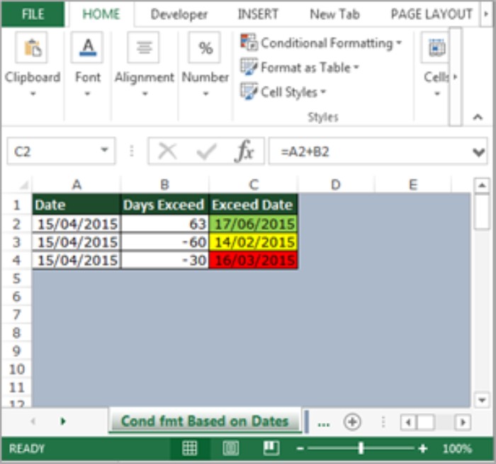
- If the date in Cell C2 is more than 60 days from today, the cell should be formatted in green.
- If the date is less than 60 days from today, the cell should be formatted in yellow.
- If the date is less than 30 days from today, the cell should be formatted in red.
This is specifically for tracking driver’s license expiration dates, aiming to receive alerts 60 days before expiration.
Follow these steps to set up Conditional Formatting:
- Select the target range for formatting.
- Click on the “Conditional Formatting” dropdown and choose “Manage Rules” to open the dialog box.
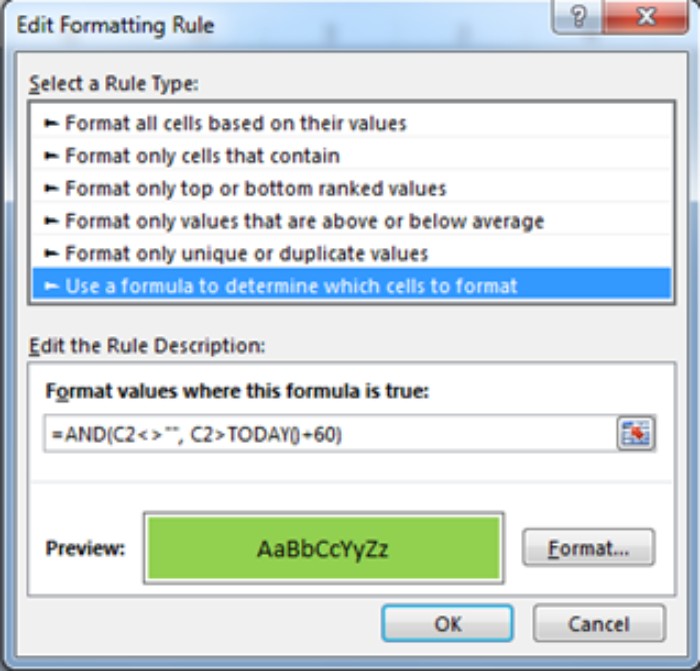
- Click on “New Rule,” and in the New Formatting Rule dialog box, select “Use a formula to determine which cells to format.”
- For dates more than 60 days from today, use the formula =AND(C2<>””, C2>TODAY()+60), and choose the green color.
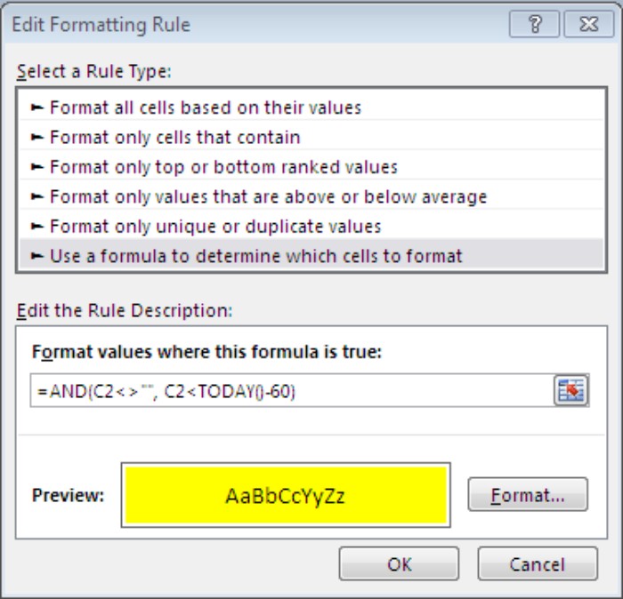
- For dates less than 60 days from today, use the formula =AND(C2<>””, C2<TODAY()-60), and choose the yellow color.
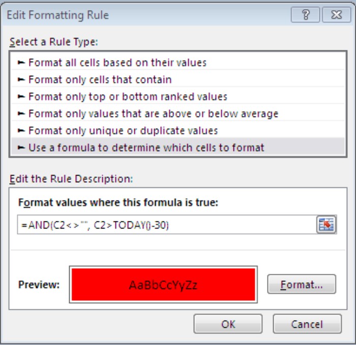
- For dates less than 30 days from today, use the formula =AND(C2<>””, C2>TODAY()-30), and choose the red color.
- Click on Apply and then OK.
Date-Based Formatting in Excel. This setup ensures a visual representation of upcoming driver’s license expirations with a color-coded system for easy identification.