
Counting Cells with Specific Criteria in Excel: A Comprehensive Guide. In this article, we will delve into the intricate process of counting cells in Excel that do not meet specific criteria. Imagine a scenario where you need to tally data based on particular conditions within an array. We’ll explore methods to count cells that don’t contain certain values, employing Excel functions and wildcards for a precise outcome.
Method 1 Counting Cells with Specific Criteria in Excel: Using SUMPRODUCT, MATCH, and ISNA Functions
This approach involves the utilization of SUMPRODUCT, MATCH, and ISNA functions to exclude specific values from the count. Here’s how it works:
Generic Formula:
=SUMPRODUCT(--(ISNA(MATCH(range, values, 0))))
Variables:
- range: Array of cells to be counted.
- values: Array of values to be ignored in the count.
Example:
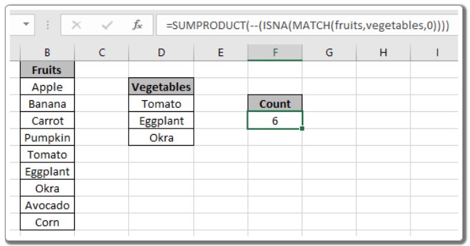
Let’s say we have a list of fruits and vegetables, and we want to count only the fruits, excluding the vegetables.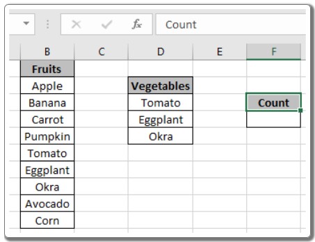
Formula:
=SUMPRODUCT(--(ISNA(MATCH(fruits, vegetables, 0))))
Explanation:
- MATCH function finds positions where values are matched in the range and returns #NA error where no match is found.
- ISNA function captures #NA errors, turning them into TRUE values, and FALSE for other cases.
- — operator converts TRUE values to 1 and FALSE values to 0.
- SUMPRODUCT function adds up these 1s and 0s, giving the count of cells where values are not considered.
Method 2 Counting Cells with Specific Criteria in Excel: Using COUNTIFS Function
For a simpler solution, COUNTIFS function can be employed to count cells that do not match specific values individually. Here’s the method:
Generic Formula:
=COUNTIFS(range, "<>value1", range, "<>value2", ...)
Variables:
- range: Array of cells to be counted.
- value1, value2: Values to be ignored in the count.
Example:
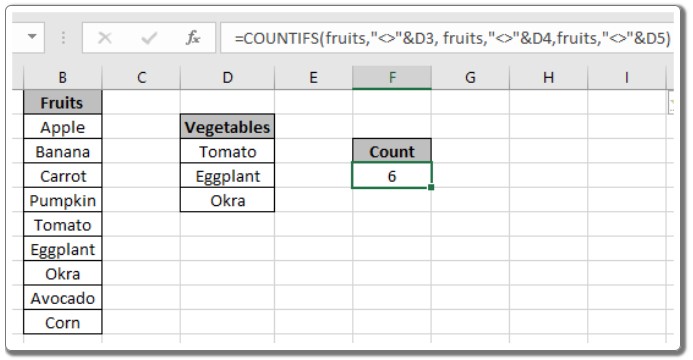
Using the same fruits and vegetables scenario, the formula can be: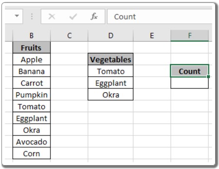
=COUNTIFS(fruits, "<>" & D3, fruits, "<>" & D4, fruits, "<>" & D5)
Explanation:
- <> operator signifies “not equal to.”
- & operator concatenates the <> operator with cell reference values.
Method 3: Employing COUNTA and SUMPRODUCT Functions
This method calculates the count of non-empty cells and subtracts the count of cells containing specific values to determine the final count.
Generic Formula:
=COUNTA(range) - SUMPRODUCT(COUNTIF(range, values))
Variables:
- range: Array of cells to be counted.
- values: Array of values to be ignored in the count.
Example:
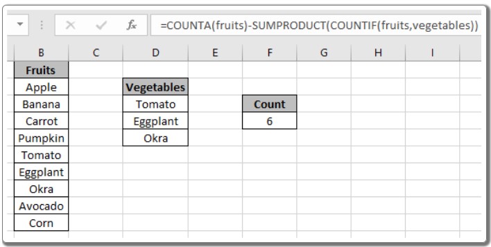
Using the fruits and vegetables example:
=COUNTA(fruits) - SUMPRODUCT(COUNTIF(fruits, vegetables))
Explanation:
- COUNTIF function counts cells in “fruits” containing “vegetables.”
- SUMPRODUCT calculates the sum considering all these values.
- COUNTA function calculates the count of non-empty cells in the range.
- The difference yields the count of cells (fruits) without the specified values (vegetables).
We hope this comprehensive guide has provided clarity on counting cells with specific criteria in Excel. For further exploration of Excel Count functions, check out our related articles. If you have any queries or feedback, please don’t hesitate to share them in the comments section below. Happy Excel-ing!


