Converting Column Letters to Numbers in Excel: A Quick Guide. We’ve previously covered converting column numbers to letters, but what about converting column letters to numbers in Excel? In this article, we’ll dive into the process of converting Excel column letters to numbers.
To achieve this, we utilize the COLUMN function, which returns the column number of a provided reference. Combining the COLUMN function with the INDIRECT function allows us to derive the column number from a given column letter.
Converting Column Letters to Numbers in Excel: A Quick Guide
The generic formula used to convert letters to numbers in Excel is:
=COLUMN(INDIRECT(col_letter & "1"))
Where:
col_letter: Represents the reference of the column letter from which you want to extract the column number.
Let’s illustrate this with an example:
Suppose we have column letters listed in cells B2:B5. Our goal is to obtain the corresponding column numbers (1, 2, 3, etc.) based on these given letters (A, B, C, etc.).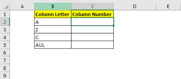
Apply the generic formula by entering:
=COLUMN(INDIRECT(B2 & "1"))
Drag this formula down through cells B2 to B5. You’ll then have the column numbers associated with the provided column letters.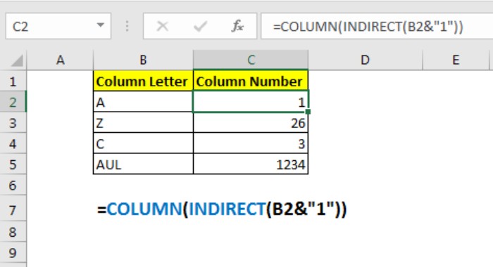
How does it work?
The process is straightforward. The key is to retrieve the reference of the first cell within the given column number. Using INDIRECT(B2&”1″) translates to INDIRECT(“A1”), obtaining the cell reference of A1.
Subsequently, COLUMN(A1) retrieves the column number associated with the given column letter.
So, that’s the method for converting a column letter into a column index number. It’s a relatively simple process. If you have any questions about this function or other advanced Excel features, feel free to ask in the comments section. Your queries are welcome!