Analyzing Actual vs Forecasted Data in Excel: A Step-by-Step Guide. Forecasting plays a pivotal role in business management, and comparing actual results with forecasts is crucial for project evaluation. Having an effective tool or dashboard to calculate variances between actual and forecasted data is essential. In this article, we will delve into the process of comparing actual and forecasted data in Excel using formulas.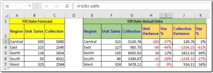
Analyzing Actual vs Forecasted Data in Excel: A Step-by-Step Guide
Generic Formula for Variance Calculation between Forecast and Actual Data
Variance = ACTUAL – FORECAST
ACTUAL: Represents the actual gathered data or amount.
FORECAST: Denotes the forecasted data or amount.
The subtraction of forecasted values from actual values helps in understanding the variance. The direction of the variance (positive or negative) indicates whether the actual values exceeded or fell short of the forecasts.
Example: Creating a Forecast vs Target Report with Variance in Excel
Let’s consider a scenario where we have sales data for stationery products in different months. By utilizing Excel forecast formulas, we have predicted sales and unit production for specific periods. As the months progress, actual sales and production data are collected in Excel. The goal is to create a report highlighting the variances between actual and forecasted values. No specialized variance formula is needed for this comparison.
- In cell H2, enter the formula to calculate unit variance:
=F3-B3
Drag this formula down to calculate variances for each period. A positive difference indicates actual units surpassing the forecast, while a negative difference signifies lower actual units compared to the forecast.
- In cell J2, compute the collection variance with the formula:
=G3-C3
Drag this formula down to calculate variances in collections.
To express these variances as percentages:
- For unit variance percentage (in column K), use the formula:
=F3/B3-100%
A negative percentage indicates a negative variance, while a positive percentage represents a positive variance.
- For collection variance percentage (in column L), apply the formula:
=G3/C3-100%
Negative values signify a negative variance, and positive values indicate a positive variance.
Additionally, you can apply conditional formatting to highlight negative values in the variance columns using red text.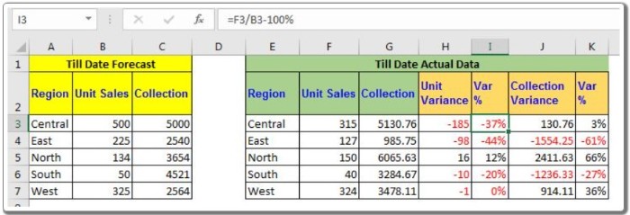
By following these steps, you can create detailed reports on actual vs forecasted data, facilitating analysis and informed decision-making. If you have specific questions about forecasting formulas in Excel or any other Excel-related queries, feel free to ask in the comments section below. Your inquiries are welcome!