Simplest Way to Obtain Relative Column Index in Excel
Simplest Way to Obtain Relative Column Index in Excel. In this guide, we will explore a straightforward method to obtain the relative column index in Excel. Often, situations arise where you need to mark the index for data in a specific column, but the data doesn’t start from the first column of the worksheet. We can solve this using the COLUMN function along with a basic logic to derive the column index in the data. Let’s delve into understanding the COLUMN function first.
The COLUMN function in Excel returns the column number of a given cell or cell reference. Its syntax is:
=COLUMN([cell_reference])
Note: If no argument is provided, the function automatically returns the column number for the cell where the formula is used.
To create our formula, we start by establishing a difference of 1 between two numbers generated by the COLUMN function. These numbers represent the current column and the column reference we want to start from. We then apply this formula across the entire table. The generic formula looks like this:
=COLUMN() - COLUMN(cell_ref)
Here’s the breakdown of the logic: Simplest Way to Obtain Relative Column Index in Excel
COLUMN()function returns the column number where it is used.- To achieve a difference of 1, we subtract the column number of the reference cell using
COLUMN(cell_ref).
Let’s illustrate this with an example: Simplest Way to Obtain Relative Column Index in Excel
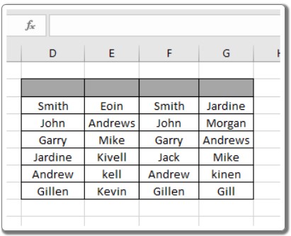
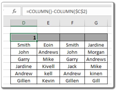
Consider a data table with names and corresponding data. We want to mark each column with its index in the given Index Row. Use the formula in cell D2:
=COLUMN() - COLUMN($C$2)
Here’s how it works: Simplest Way to Obtain Relative Column Index in Excel
COLUMN()returns 4, the column number for cell D2.COLUMN($C$2)returns 3, the column number for column C (our reference column).- The fixed reference using the
$sign ensures the correct calculation across the cells.
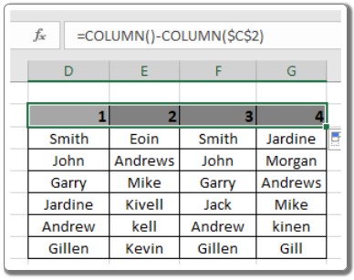
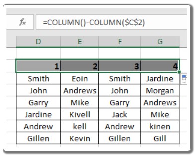
Upon entering the formula, you will notice that the first index for the table is correctly marked as 1. Copy the formula to other cells using the Ctrl + R shortcut or Excel’s drag-right feature.
Alternatively, if you are using Excel 2016 or later versions, an even simpler method is available. Just type 1 and 2 in the first two index spaces, select the cells, and drag them right from the bottom until the column index is populated automatically.
This method ensures that your index column is efficiently filled with the desired values. We hope this guide has clarified how to obtain the relative column index in Excel. For more Excel-related tips and tricks, explore our articles on Excel cell reference functions. If you have any questions or feedback, feel free to reach out.


